Machine Learning Foundations for Product Managers Wk 6 - Capstone
- Muxin Li
- Jun 15, 2024
- 9 min read
Updated: Jun 25, 2024
We take everything we've learned in Machine Learning for Product Managers and apply them to a real-world scenario: Building a model to predict the power output of a power plant.
What's Covered:
Project details and background
How to work through the project step by step
Training, Validating, and Testing
Evaluation of machine learning models
Full Python code to train and evaluate models on your own
Key takeaways:
Understanding the context of the problem you're trying to solve is of critical importance in order to select the right modeling approach.
Before jumping straight into trying different models on your dataset, first understand how potential features interact and impact the target output.
There is no free lunch - each model has pros and cons. The final model you will need in the real world will depend on your use case. Always involve stakeholders and relevant subject matter experts in discovery and requirements building, just like you would in creating a PRD.
Table of Contents
Let's get started!
The Problem
(From the Course details):
In this project we will build a model to predict the electrical energy output of a Combined Cycle Power Plant, which uses a combination of gas turbines, steam turbines, and heat recovery steam generators to generate power.

We have a set of 9568 hourly average ambient environmental readings from sensors at the power plant which we will use in our model.
The columns in the data consist of hourly average ambient variables:
- Temperature (T) in the range 1.81°C to 37.11°C,
- Ambient Pressure (AP) in the range 992.89-1033.30 milibar,
- Relative Humidity (RH) in the range 25.56% to 100.16%
- Exhaust Vacuum (V) in the range 25.36-81.56 cm Hg
- Net hourly electrical energy output (PE) 420.26-495.76 MW (Target we are trying to predict)
Guidelines for the project:
To complete the project, you must complete each of the below steps in the modeling process.
For the problem described in the Project Topic section above, determine what type of machine learning approach is needed and select an appropriate output metric to evaluate performance in accomplishing the task.
Determine which possible features we may want to use in the model, and identify the different algorithms we might consider.
Split your data to create a test set to evaluate the performance of your final model. Then, using your training set, determine a validation strategy for comparing different models - a fixed validation set or cross-validation. Depending on whether you are using Excel, Python or AutoML for your model building, you may need to manually split your data to create the test set and validation set / cross validation folds.
Use your validation approach to compare at least two different models (which may be either 1) different algorithms, 2) the same algorithm with different combinations of features, or 3) the same algorithm and features with different values for hyperparameters). From among the models you compare, select the model with the best performance on your validation set as your final model.
Evaluate the performance of your final model using the output metric you defined earlier.
Follow Along with Dataset and Python Code
Store both of these files in the same folder. Otherwise, you'll have to update the Python code with the correct directory path of the CCPP dataset CSV file.
Copy of our project dataset
Full Python code to follow along
Note - You will need to convert this to Python file by replacing 'txt' from the file name with 'py'.
You will also need to have Python set up on your computer. On ChatGPT or your favorite LLM chatbot, enter this in the prompt:
Hello! I need help setting up Python on my computer. Can you guide me through the entire process, including downloading and installing Python, setting up a development environment, verifying the installation, and running a basic Python script? I am using [specify your operating system: Windows/macOS/Linux]. Additionally, could you recommend some good code editors or IDEs for Python development and show me how to install and use packages with pip? I want to ensure everything is set up correctly for me to start coding in Python. Thank you!
You will need to install the following Python libraries to be able to run the code:
psutil: This library provides an interface for retrieving information on system utilization (CPU, memory, disks, network, sensors) and system uptime.
pandas: This library is used for data manipulation and analysis, providing data structures and operations for manipulating numerical tables and time series.
scikit-learn: This library includes simple and efficient tools for data mining and data analysis. It is built on NumPy, SciPy, and matplotlib.
If you get stuck or run into errors, ask your friendly AI chatbot!
Step 1 - ID Output Metric and the Approach Needed
This is a regression problem - we're trying to calculate the produced energy output of a combined cycle power plant based on a set of sensor data - the output is going to be a continuous number like 420.26 MW.
For regression related Output Metrics, we're using Mean Squared Error and R-Squared to evaluate the overall model - MSE for accuracy and R-squared for how well the model explains how good of a fit the model is.
We can also use R-Squared for each of the input features, to better understand how correlated each of those features are to the energy output of the plant. If there are features that aren't strongly correlated to the target output, we may consider removing them to reduce the complexity of the model.
However, we're going to start off by trying all the features first.
Step 2 - ID the Features and Models
Luckily, we already have a list of features included in our dataset:
- Temperature (T) in the range 1.81°C to 37.11°C,
- Ambient Pressure (AP) in the range 992.89-1033.30 milibar,
- Relative Humidity (RH) in the range 25.56% to 100.16%
- Exhaust Vacuum (V) in the range 25.36-81.56 cm Hg
- Net hourly electrical energy output (PE) 420.26-495.76 MW (Target we are trying to predict)
Later on, we'll redo the analysis with a reduced feature set and only keeping the highest correlating features that explain the output.

For model selection, we need a better understanding of how these features affect the target output. How complicated is the relationship between ambient environmental variables on the energy output of a combined cycle power plant?
It turns out that not only do all of these variables affect the electricity energy output, but they also affect each other:
In a combined cycle power plant, the ambient environmental variables (temperature, pressure, relative humidity, and exhaust vacuum) can indeed affect the net hourly electrical energy output. Moreover, these variables can also influence each other, creating a complex set of relationships.
Here's a high-level summary of these interactions:
Temperature (T):
Higher ambient temperatures generally lead to lower power output. This is because the gas turbine's efficiency decreases as the inlet air temperature rises.
Temperature can also affect relative humidity, as warmer air can hold more moisture.
Ambient Pressure (AP):
Higher ambient pressure typically results in higher power output. Increased air density at higher pressures allows the gas turbine to compress more air, leading to better efficiency.
Pressure can be influenced by temperature, as warm air tends to rise and create areas of low pressure.
Relative Humidity (RH):
High relative humidity can slightly decrease power output. Moist air is less dense than dry air, which can reduce the mass flow rate through the gas turbine.
Humidity is directly affected by temperature, as warmer air can hold more water vapor.
Exhaust Vacuum (V):
A higher exhaust vacuum generally improves power output. The vacuum helps to remove exhaust gases more efficiently, maintaining optimal flow through the turbine.
The exhaust vacuum can be influenced by ambient pressure, as a higher ambient pressure can make it more difficult to maintain a strong vacuum.
Net Hourly Electrical Energy Output (PE):
This is the target variable you are trying to predict, and it is affected by all of the above factors.
In general, lower temperatures, higher pressures, lower humidity, and higher exhaust vacuum contribute to increased power output.
So not a simpler multiple linear regression model, then. Since each feature can also affect each other, we need something more robust that can handle the additional complexity, like Ridge Regression, which is capable of handling multi-collinearity (when there are relationships/correlations between input features to each other).
Another model that's capable of handling complex relationships between input features are ensemble models - the Frankenstein's Monster of model builds. The ensemble model that we've covered in this course, which is capable of handling regression problems, is a Random Forest - a collection of decision trees working together to minimize the decision tree tendency to overfit to their training data.
Step 3 - Validation Strategy and Data Splitting
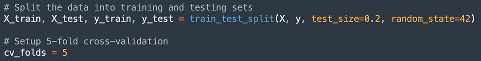
We'll split the data into 80% for training and 20% for final Testing. During training, we'll run a K-Folds Cross Validation (K = 5) to fine tune each model's hyperparameters so that we're comparing a tuned up version of each model against each other before selecting the best one.
Step 4 - Training and Test Results
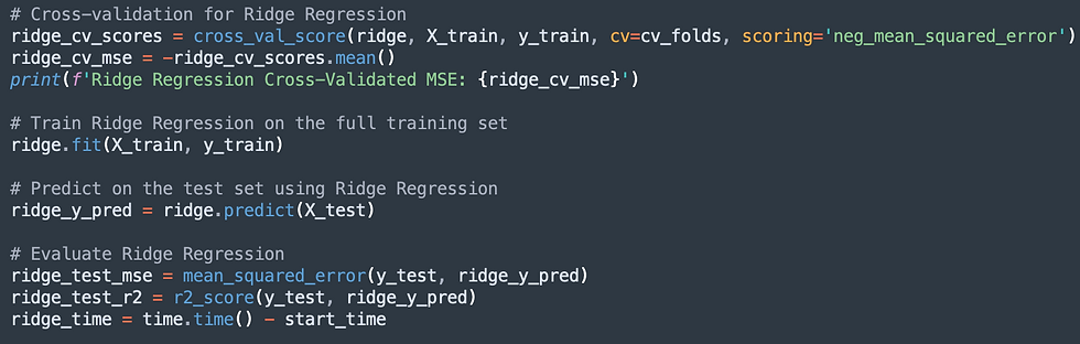
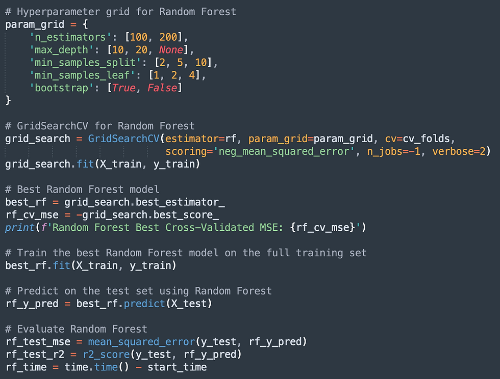
Thanks to the scikit-learn Python library, we're able to run the validation process automatically, updating coefficients and hyperparameters to fine tune our selected models.
Results and Evaluation
Below are the output metrics (MSE and R-Squared) from running Ridge Regression and Random Forest models on 80% split data for Training-Validation, and 20% split data for final Testing:
Cross-Validated MSE | Test Set MSE | Test Set R-Squared | |
Ridge Regression | 20.92 | 20.27 | 0.9301 |
Random Forest | 11.92 | 10.43 | 0.9640 |
Winner | Random Forest | Random Forest | Random Forest |
Interpreting the results:
Cross-Validated MSE: The Mean Squared Error (MSE) averaged over the 5 folds during cross-validation. It indicates the average error when the model is applied to unseen data in each fold. The lower the better.
Test Set MSE: The MSE when the model is applied to the test set. It shows the average squared difference between the actual and predicted values on the test data. The lower the better.
Test Set R-Squared: The R-squared value indicates how well the model explains the variability of the target variable. A value of 0.9301 means that approximately 93% of the variability in the power output can be explained by the model. The higher the better.
Step 5 - Final Model Selection
However, accuracy isn't everything. If we want to apply a model to the real world, we should evaluate other factors:
How much compute resources does the model use? Is it cost efficient to run?
How fast do we need the model to be in a power plant?
Do we care about interpretability, or how easy the model is to explain?
Evaluating Model Performance
We can use the Python library psutil to calculate standard compute resource usage of each model - here are the results from running Ridge Regression vs Random Forest on compute usage and speed:
Ridge Regression | Random Forest | |
Training Time | 0.006 seconds | 126.93 seconds |
CPU % | 2.94% | 2.23% |
Memory RSS | ~146.6 MB | ~456.4 MB |
Memory VMS | ~422.5 GB | ~423.1 GB |
User Time | 1.04 seconds | 7.09 seconds |
System Time | 4.29 seconds | 4.59 seconds |
Conclusions | Fastest, fewer compute resources, but less accurate | Slower, but more accurate |
Explaining the Results:
Training Time: The time to train the model.
CPU Percent: How much of the CPU’s power the process is using right now. A value of 0.0 either means it's negligible, or it didn't read due to the timing of the measurement.
Memory RSS: The amount of physical memory (RAM) the process is currently using.
Memory VMS: The total memory the process could potentially use, including RAM and virtual memory on disk. It’s the maximum space the process could potentially use.
User Time: This is the amount of time the CPU has spent running the process's code. Higher values mean the process is doing a lot of computations.
System Time: the amount of time the CPU has spent doing system-related tasks for the process, like reading files or handling network requests. Higher values mean the process is making the system do a lot of work.
Conclusions
Which model is the best will ultimately depend on the use case - if used for real-time monitoring, then Ridge Regression is the clear winner. If accuracy is more important and speed is not an issue, then Random Forest is a better choice. For interpretability, Ridge Regression is easier to explain, however in this scenario the value of interpretability is debatable (unlike in decision making over home loans or job applicants).
The best way to understand how important these factors are is to interview experts and relevant stakeholders.
Bonus! Testing with Fewer Features
Reducing the number of features we evaluate will reduce the model's complexity, which can allow for better model performance. Let's try it!
We'll first run a multi-correlation analysis in Python on all the features and the output target (PE). Here are the results - 1 is a perfect correlation:
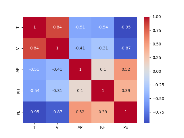
RH/Relative Humidity and AP/Ambient Pressure are less impactful features to our output metric, PE/Hourly electrical power output. They also have weaker correlations to other input features.
Let's try removing those features from the dataset and rerun our models again, and see if it's moved the needle on our output metrics MSE and R-Squared:
Reduced Feature Set | Cross-Validated MSE | Test Set MSE | Test Set R-Squared |
Ridge Regression | 24.67 | 24.07 | 0.9170 |
Random Forest | 14.33 | 13.48 | 0.9534 |
Winner | Random Forest | Random Forest | Random Forest |
VS Previous outputs with all input features:
Original Feature Set | Cross-Validated MSE | Test Set MSE | Test Set R-Squared |
Ridge Regression | 20.92 | 20.27 | 0.9301 |
Random Forest | 11.92 | 10.43 | 0.9640 |
Winner | Random Forest | Random Forest | Random Forest |
Although RH and AP were weak features, the results prove they did provide some value in increasing the performance of the models. This is in line with real-world examples of weak features being used in AI-powered finance startups like Smart Finance, described in AI Superpowers - Smart Finance successfully uses many weak features to improve their lending prediction AI models.
Like this post? Let's stay in touch!
Learn with me as I dive into AI and Product Leadership, and how to build and grow impactful products from 0 to 1 and beyond.
Follow or connect with me on LinkedIn: Muxin Li
Comments