Technical terms:
Neural Networks
Deep Neural Networks
Deep Learning
Perceptron
Threshold Function
Logistic Regression
Activation Function
Forward Propagation
Backpropagation
Gradient Descent
Vectorized Operations/Vectorization
Stochastic (SGD)
Batch
Mini-batch
Vanishing Gradient
Recurrent Neural Networks (RNN)
Long-range Dependencies
Multilayer Perceptron (MLP)
Fully connected layers
Transfer Learning
Convolutional Neural Networks (CNNs)
Convolutional Layers
Pooling Layers
Natural Language Processing (NLP)
Transformers
Positional encodings
Attention mechanisms
Neural Networks
A quick history on neural networks and deep learning - the idea of using our brains as a guide for creating complex computation models officially started in 1943 with Warren McCulloch (neurophysiologist) and Walter Pitts (mathematician). However, research progress stalled in the 70s and 2000s ('AI Winters') - until increase in labeled data available for training, algorithmic advances and computing power increased tremendously to allow for far more complex modeling.
Neural networks at its core operates by connecting many artificial neurons - the computational model developed to mimic how our brains' neurons work:
Signals arrive through the dendrites - if the total of signals exceeds a threshold, the neurons are activated and passes an output signal.
Imagine thousands of these neurons interlinked together, firing output signals off to each other based on input signals, and woven into a network.
Imagine networks working with other networks through layers - one layer handles inputs, many hidden layers handle the computation, another layer handles the outputs.
Simpler neural networks are just 'neural networks' with 1-2 layers.
Deep Neural Networks (DNN) is a more complicated type of neural network, with multiple hidden layers (usually 3 or more). All DNNs are neural networks, not all neural networks are DNNs.
Deep learning (a subset of neural network) uses many layers of interconnected nodes of data - more layers allow for more complex and abstract jobs, like recognizing images. These layers can be made of neural networks, or they can be made of a combination of neural networks and attention mechanisms like in Transformers architecture, which power AI models like OpenAI's GPT or Anthropic's Claude.
Artificial Neurons
It all started with mimicking a simple neuron, firing output signals based on whether its accumulated signal (from dendrites) exceeded a threshold:
Come to think of it, this process sounds a lot like a classification problem - the scenario being, 'should this neuron fire an output signal or not - yes or no'?
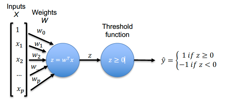
That's essentially what the perceptron does, a basic artificial neuron that sums up a set of weighted features, passes it through a threshold function to determine of the threshold is exceeded (in this case, if the sum of weighted inputs is 0 or higher), then 'activates' the neuron aka fires the output signal.
Taking us all the way back to Module 4 on Linear Models, this looks very similar to using a logistic regression model for classification problems:
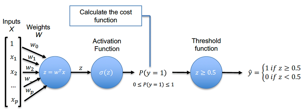
In fact, another artificial neuron is the logistic regression - similar to the perceptron model but with the addition of an activation function (using the sigmoid function formula):
Sigmoid/Activation Function will take the calculate the probability of our classification being a yes (1) or a no (0) based on the sum of the weighted inputs.
The output of the Activation Function then goes through the Threshold Function, which we can set by design, and that determines of the probability is high enough to fire an output signal in our artificial neuron.
Training Artificial Neurons
The goal of a good model is to increase its accuracy in making predictions - in this case, it means to increase the probability score that's calculated by our Activation Function so that we get a higher chance of hitting our threshold. This means adjusting weights of our inputs (or even our inputs entirely) to get a higher probability, since those weighted inputs are what feeds into the Activation Function.
Usually if you have the wrong features, that means you didn't understand the problem correctly - maybe the number of pet stores in a 1 mile radius didn't really matter to the price of a home. Use the CRISP DM process in Module 1 whenever you're starting out with a new domain problem, and check with experts to better understand which features are the most important.
In this exercise, we're focusing only on figuring out what weights to use and leaving the features alone.
Improving model performance means minimizing its cost function - here's where it diverges from the course content a bit. For logistic regression models, the consensus is using the log loss/binary cross-entropy as the cost function - it takes the probabilities calculated by the Activation Function/sigmoid, applies natural logarithm to them, then sums up and averages the log values to get the log loss (for convenience, you may take the absolute value of the output to get a positive number). More in-depth details for the mathematically curious.
The main takeaways are the basics behind training artificial neurons, the pros and cons of different ways to feed the model data, and some of the parameters to be mindful of.
Training through Propagation and Iterating with Gradient Descent
Minimizing the cost function means to take its derivative and set it to 0, then work backwards towards the weights you need to achieve that result (a closed-form solution - like a more advanced algebra problem where the output is 0).
That works for linear regression, but logistic regression models won't work that way - we need an iterative process, which is prime time for using gradient descent.
We calculate the cost, move towards the minimum (opposite of the derivative of the cost function), and once we've arrived at the minimum we then solve for the weights or the coefficients of our inputs. This process will be affected by the learning rate that we set.
A detailed outline of gradient descent is in Module 4
The overall process for training will look like this - this assumes you have pre-labeled data and desired outputs for your model:
Forward propagation: Run the model on your inputs and starting coefficients/weight and get your initial outputs.
For each weight, calculate the cost of your model's output vs the correct answer (using the log loss function since this is a logistic regression model). Calculate the derivative as well.
Backpropagation: Now update each of those coefficients using the gradient descent process. The new weight value = Previous Value - learning rate * derivative of the weight's cost function.
Step 2: Calculate the gradient of the cost function with respect to each weight
New weight coefficient values (note: 'gradient' and 'derivative' get used interchangeably):
Methods for Gradient Descents and Feeding Data
Deciding how much data to feed into the iterative process of gradient descent can depend on your needs.
Vectorized Operations/vectorization is a powerful way to speed up calculations by using arrays or matrices instead of individual elements. However, not every method of gradient descent can use this.
Stochastic Gradient Descent (SGD) | Batch Gradient Descent (BGD) | Mini-batch | |
|---|---|---|---|
Methodology | Runs the training process one data point at a time, each time updating your model. | Uses the entire dataset to calculate the weights to update your model. | Compromises by creating smaller batches of training data to train the model. |
Pros | Faster than batch gradient descent, especially in large datasets. Better at avoiding false 'local minima' that aren't the true minimum of your gradient descent. The randomness in each data point can help the model 'jump out' of local minimas. | Can use vectorized operations to speed up calculations. Most likely to find the global minimum of a smooth, bowl-shape curve/aka convex loss functions with 1 minimum - with a good learning rate. | Can use vectorized operations, and can work well with large datasets. Most practical choice compromise between speed and accuracy - less noisy than SGD, can work with larger datasets than BGD. |
Cons | Cannot use vectorized operations - by definition, SGD loops through each element at a time. Settles for a good enough minimum and may not find the absolute best, global minimum. | Computationally expensive for large datasets, as it requires loading the entire dataset into memory. Can be stuck in a local minima for convex loss functions that have many 'dips'. | Tweaking hyperparameters becomes more important - determining the size of each mini-batch, the learning rate. Can still be stuck in a local minima (but less than BGD). |
When to Use | Massive datasets and sparse datasets - using batch in massive datasets is too computationally expensive, but using SGD can get you quickly to a good enough solution. Speed is top priority - good for Online learning (e.g. predicting stock prices), where data is constantly streaming in and the model needs to update with each new datapoint. | Smaller to medium sized datasets (but not sparse - enough to be usable). For when you have smaller datasets and need more accuracy than speed. Fixed datasets that are static and unchanged - image classification, spam detection, sentiment analysis.. by definition, the entire pre-labeled dataset is used for training in batches. | Medium to larger datasets, but is a good default starting point for most scenarios. Non-convex (non-bowl-shaped) loss functions with some local minima. Fixed datasets running on GPUs. Most modern ML models use a mini-batch method. |
Learning Rates and Vanishing Gradients
A quick review on learning rates and their impacts on gradient descent - picking the right learning rate matters to achieve results in a reasonable time.
In deep neural networks, the gradients can become too small to make noticeable updates to the model via backpropagation - this vanishing gradient problem can occur from networks getting too deep (and needing more multiplications of derivatives - if derivatives are small, the resulting gradient calculated from them will get even smaller very quickly).
Slow learning leads to slow model improvement - or even none at all.
The model is unable to update deeper layers, making it unable to handle more complex tasks.
This challenge tends to occur for recurrent neural networks (RNNs), which analyzes sequential data like text and stores in its memory the information it captures along each step. The vanishing gradient problem creates memory challenges for RNNs to be able to handle long-range dependencies, or the relationships and context between elements that are separated by a significant distance in a sequence.
Transformers can significantly mitigate the vanishing gradient problem and long-range dependencies via attention mechanisms, though they don't get rid of it completely.They can weigh the importance of different words in a sentence relative to each other, regardless of their position, allowing for more nuanced understanding of context and meaning over long sequences
Building up to Neural Networks
A single neuron only handles 1 linear decision - adding these simple artificial neurons together allow for more complex tasks.
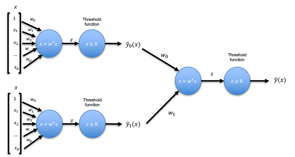
A multilayer perceptron (MLP) is exactly that - multiple layers of perceptrons (basic artificial neuron) connected together.
Below, we take the outputs of 2 perceptrons and feed those as inputs to a 3rd perceptron.
Classifying multiple things with MLPs
MLPs can be used to solve multiclass problems like, 'ID all the different flower species' by including multiple output layers.
Input layers made of our input features feed into hidden layers that then feed into the output layers, which assigns a score for the different classes. The class with the highest score becomes the label for the input datapoint - e.g. 0.8 class 1, 0.1 class 2, 0.1 class 3 = assign label for class 1 to datapoint fed to the model.
Below is a simple 3-layer network with 3 class outputs.
These types of networks are also called fully connected layers - each value from a previous layer is connected to a subsequent layer.
Each layer's threshold function calculates what the inputs are to the next layer (or the final output) - the example above seems to be using a simple sum of all weighted inputs. We can also decide to change formulas used between each layer's threshold function to model non-linear relationships.
So in the below example, we've replaced the simpler threshold function used in the hidden layers and the output layer with something less simple (looks like a sigmoid?):
Training Neural Networks
Training a whole network is a lot like training an artificial neuron - we run the model, calculate the cost, do the gradient descent to find the minimum and update the coefficient or weight values of the inputs.
Shortcuts to Training Neural Networks
There's lots of decisions that can impact the performance of a neural network - how many layers? How many neurons per layer? What's the activation function per layer? Which method of gradient descent? What's the learning rate?
You could either use a neural network that's too big for your problem ('stretch pants') and size it down to fit the data and problem you have, or you can use transfer learning and start by using a pre-trained model that you then fine tune for your needs (do this one).
Thanks to awesome researchers, there are pre-built, pre-trained neural networks for different tasks - find the one relevant to your problem e.g. classifying flowers.
You can take out some of the final output layers of the generic model, splice it with the layers you have built out, then train those new layers on your specific dataset (types of flowers).
Computer Vision
How did scientists teach computers to see? Each pixel can be represented as a number - e.g. RGB is a common color encoding for red, green, blue values on a scale from 0 to 255.
For any image, each pixel can be encoded using RGB. Imagine a gigantic matrix with each row and column determined by the number of pixels, and an RGB value in each 'cell' - once encoded, this gets fed into a model.
That can be a LOT of coefficients/weights and features to evaluate. To handle this, convolutional neural networks (CNNs) are needed - these use convolutional layers to act as filters for identifying patterns, and pooling layers to reduce dimensions (which reduces complexity).
What? As far as I can tell, CNNs uses filtering to see different aspects of images, then uses pooling to 'summarize' the most important aspects so the model isn't overwhelmed by too much info.
CNNs are great at various vision tasks:
Image classification - ID this picture, facial recognition.
Object detection - Where are the objects in the image.
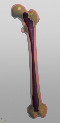
Semantic Segmentation - Classify each pixel within an image - e.g. 'is this bone or tissue' in the image below.
Image generation - self explanatory.
CNNs can tell this is a bone (image classification) as well as which parts are the bone vs tissue (semantic segmentation).
Natural Language Processing (NLP)
Like computer vision, we need a way to turn text into numbers in order to feed it to teh computer model. The main ways to do this:
Bag of words - taking a survey of the different words in our vocabulary and counting the number of times they're used.
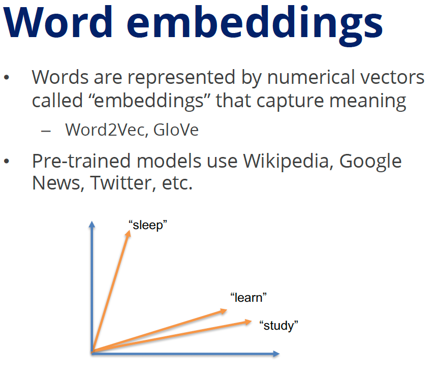
Embeddings - in pre-trained models like Word2Vec and GloVe, similar words are closer to each other and assigned numbers.
Transformers - uses a combination of embeddings, positional encodings (where is the word located in the sentenced, encoded into a number), and attention (how strongly words in sentences are related to each other, also a number).
Pros and Cons of Neural Networks
Modeling very complicated relationships, large number of features, and excellent with unstructured data - neural networks need little (often no) feature engineering work to figure out which features to feed. It's also gotten easier to work with neural networks thanks to modern tools like Google ML.
However, they are computationally expensive to run - very large amounts of calculations are needed, requiring lots of compute resources (and energy to power those super computers). They can be difficult to train, are difficult to interpret (what is going on in those hidden layers?), and they can easily overfit to small datasets.
Transparency into how these models work can matter a lot if you're deciding who should get a home loan or be admitted to grad school. Ethical considerations towards interpretability need to be accounted for when selecting the right model to use for the problem domain.
Congrats on making it this far!

You deserve a treat - you've earned it.
That wraps up Machine Learning Foundations for Product Managers. Next post will cover the Capstone Project and applying what we've learned to a dataset.
Like this post? Let's stay in touch!
Learn with me as I dive into AI and Product Leadership, and how to build and grow impactful products from 0 to 1 and beyond.
Follow or connect with me on LinkedIn: Muxin Li








Comments